[ultimate_heading main_heading=”Web-based application for advanced mass spectra analysis using your own database of ions” main_heading_margin=”margin-bottom:10px;” main_heading_style=”font-weight:bold;” main_heading_font_size=”desktop:50px;” main_heading_line_height=”desktop:60px;”]The main advantages is that the user can generate his own database in a google spreadsheet format. As example, you can see the “easycont” spreadsheet to track common ESI and MALDI-MS contaminants  and background ions inherent to the sample preparation, such as detergents, polymers, contaminants from containers and solvent interference. The application compares the experimental spectrum to theoretical ions and calculates similarity scores based on the whole isotopic pattern. In a few seconds, the final result is a table with a list of identified known pollutants present in the sample and the annotated mass spectrum.Similarly to all the other applications of our mstoolbox,  the calculations are performed locally in the browser, with no data transferred to the servers.[/ultimate_heading]
app-7
Generate the Molecular formula or isotopic distribution of any molecule here.
Details
app-13
Generate your own database and match it in a simple click with your experimental mass spectra.
Details
app-index-app2
Find other open access applications for mass spectra interpretation.
Details
[ultimate_heading main_heading=”How to create your custom database step by step” main_heading_margin=”margin-bottom:10px;” main_heading_style=”font-weight:bold;” main_heading_font_size=”desktop:50px;” main_heading_line_height=”desktop:60px;”]Check related concepts in our glossary[/ultimate_heading]

Step 1

Create your own Google Spreadsheet file

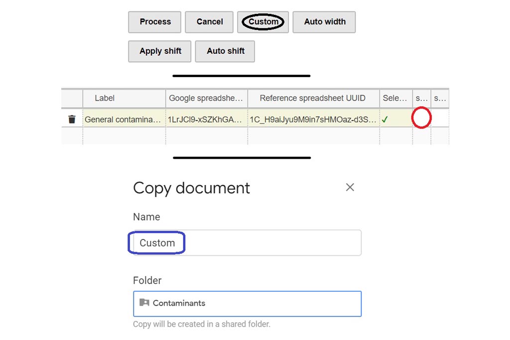
First you must click on Custom button signaled in the figure as a black oval (1). In the custom module you have to open the existing google spreadsheet signaled in the figure as a red circle (2). Once open, go to file and make a copy, change the name signaled as a blue rounded rectangle (3) and folder. Then, you can delete raws and start your own DB from scratch by entering your own compounds.

Step 2 (mandatory)

Entering your own compounds

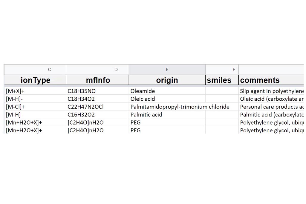
As you can see in the demo google spreadsheet, you must define the molecular formula in the first raw and how the molecule can be cationized in the second raw. This tool allows multiple entries per raw. For example, a PEG compound is a pollutant with a H-(C2H4)1-20-OH structure that can be cationized by H+, Na+ and K+ (raw 71 in the example google spreadsheet). This tool generates all the possibilities of PEG contaminant ions (20*3=60) and produces their Molecular Formula taking into account their charges and their isotopic distribution. Any group & number can be defined in here.

Step 3 (optional)

Information details

Even if this step is not mandatory, the authors highly recommend to fill it because (1) Once your database is generated you can use it as many times as you want, you can change it or you can share it but sometimes the information (origin, etc…) about a molecule might be lost. All the information will be showed in the info view (Results 3). You could specify the type of ion, the molecular formula info, the origin of the molecule, references but also some personal comments.

Step 4

Getting the UUID

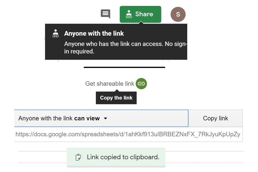
Once your google spreadsheet is saved, click on “get shareable link” with anyone  or with only defined users. When the clipboard is pasted, you must obtain something like this:

https://docs.google.com/spreadsheets/d/1ahKkf913uIBRBEZNxFX_7RkJyuKpUpZyBy-8VDGBvs4/edit?usp=sharing

Copy the bold & italic part of the link under the column “Google spreadsheet UUID” in the custom module. Then you can label your database, and add some references if needed.

Step 5

Selection of your custom database

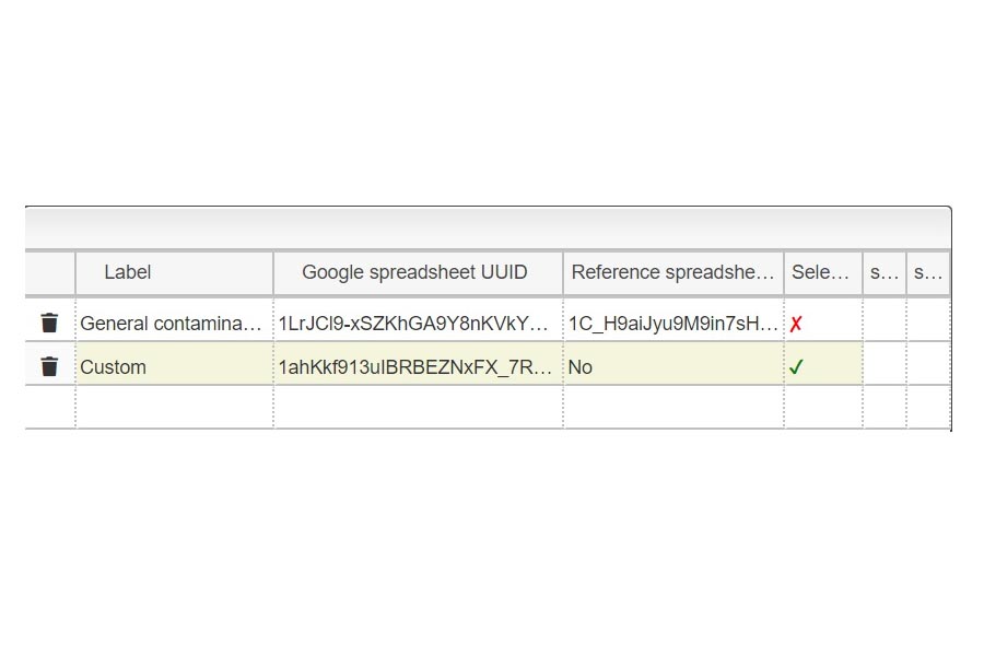
When you paste the shareable link in the UUID column, all your compounds will be automatically loaded in the list of possible molecular formula. Then you just click in the column “selected” and a green mark turns on. Finally you must click on back home. The software will use the selected custom database for further calculations.

[ultimate_heading main_heading=”How to compare experimental data with my own database step by step” main_heading_margin=”margin-bottom:10px;” main_heading_style=”font-weight:bold;” main_heading_font_size=”desktop:35px;” main_heading_line_height=”desktop:60px;”][/ultimate_heading]

Step 6

Importing Experimental data or use Easycont

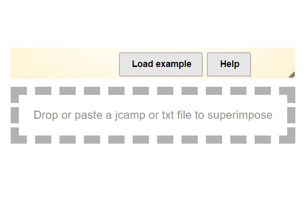
This tool can be either used in a LIMS or stand-alone. In the stand-alone mode you should either drag/drop your experimental spectrum as a tab-delimited text file or copy paste it (CTRL-V) while moving you mouse over the drop zone. The list of available spectra will be displayed in the table and you may click on one of them to display it. If you need to probe background ions, you can charge our easycont database which allows a fast identification of contaminants in HR-MS spectra. As an example you can view a mass spectrum of a contaminated samples by clicking on Load.

Step 7

Peak width picking

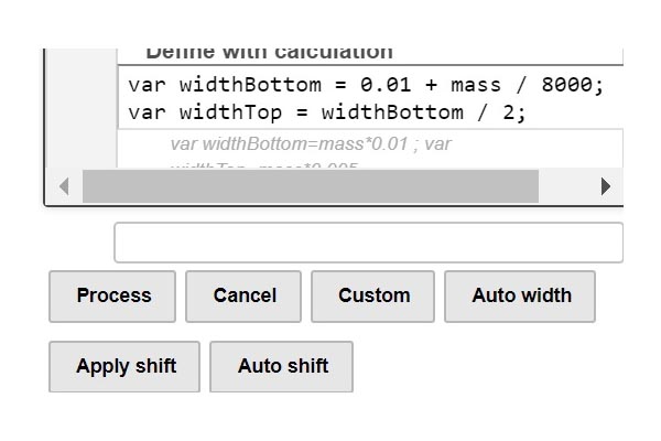
Once the experimental spectrum is uploaded, you need to click Auto width to calculate the resolution as a function of the m/z and generate the corresponding regression curve used to adjust the peak width. The result is automatically displayed in the “Define with calculation” window, then process your spectra as usual.

STEP 8

Select the matching threshold

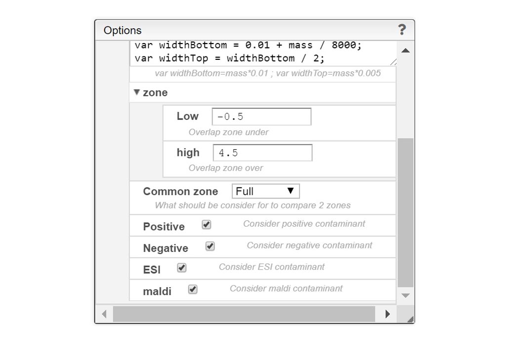
In order to improve the isotopic profile matching between theoretical and experimental data a few spectrum filters should be properly set here. First you should set the comparison zone which is the zone that will be considered to evaluate the similarity. Secondly,  set the comparison zone which should be adjusted based on the complexity of the expected isotopic pattern. If you don’t want to apply any correction click in the process button. 

STEP 9 (Optional)

Apply a correction

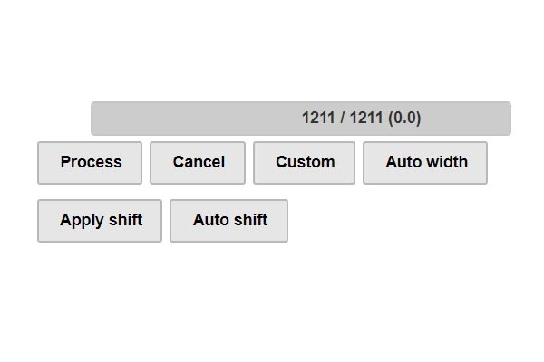
In order to improve the similarity calculation, optionally we could apply a manual Shift. The user can manually define a shift in Da in the shift window and apply it. Then you can run the calculation clicking process. In the auto-shift button when a first process is done and similarities calculated, all the best matches (similarities > 80%) are taken and the median value of their mass error calculated. This value is displayed in Da in the “shift” window, then PROCESS again to apply this shift and calculate new similarity scores.

[ultimate_heading main_heading=”Different output views in database” main_heading_margin=”margin-bottom:10px;” main_heading_style=”font-weight:bold;” main_heading_font_size=”desktop:35px;” main_heading_line_height=”desktop:60px;”][/ultimate_heading]

Results 1

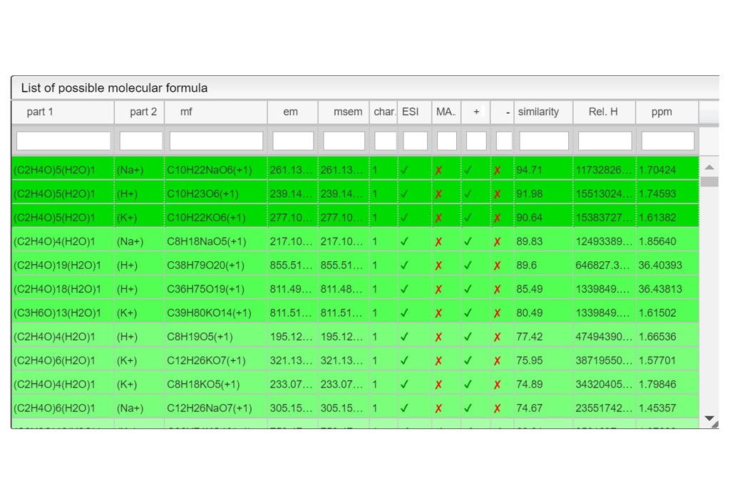
List of Possible molecular formula view

The first view is a summarizing table named List of possible molecular formula. It contains all the information about the identified peaks.You can see the containing parts, the molecular formula and its ionization form, the Molecular formula monoisotopic peak (without ionization) and the final monoisotopic mass including the charge. Another interesting values such as the mass error in ppm and the similarity score are also included in this view. All the data presented in the table can be classified by any criterion with a simple click on the column header. You can also use the search bar in order to search faster an individual value or use it by range (go to glossary). You can also export the whole table as text file with Export Data button.

Results 2

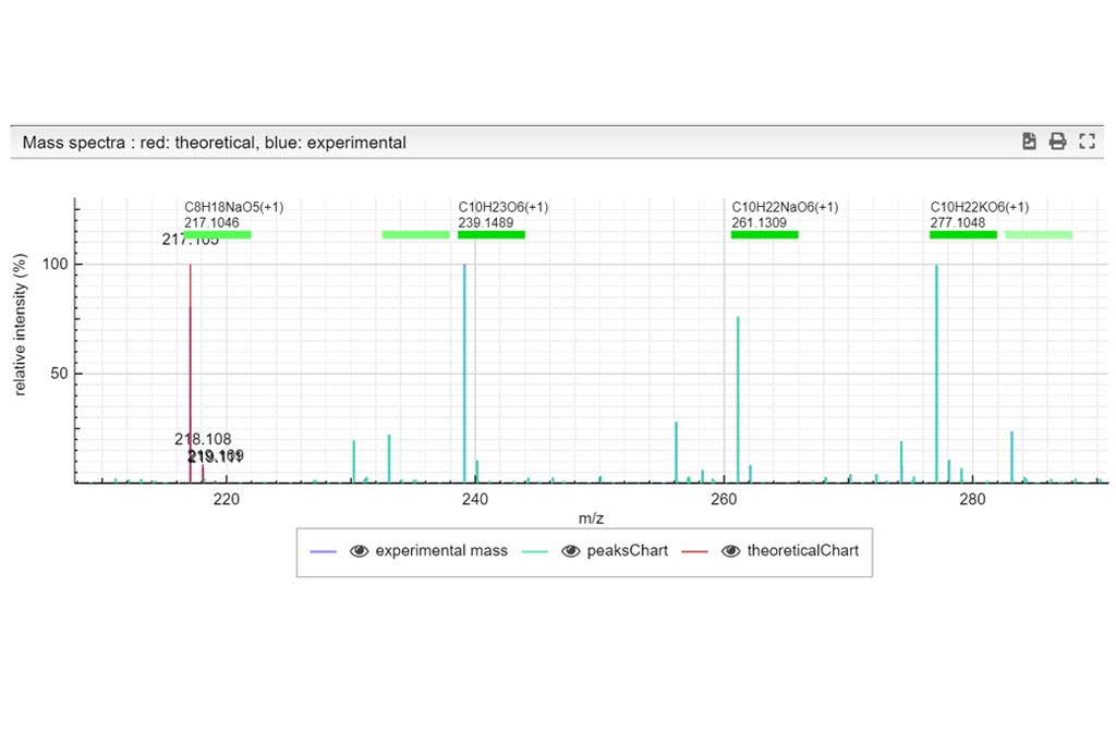
Mass spectra view

The Mass spectra window displays the experimental data (in blue) overlaid with the theoretical matched peaks (in red). Identified ions are assigned  with details on the top (molecular formula). You can select a single ion in the table view (Results 1) and it will be highlighted in this view (in red). It is possible to zoom in (left button), zoom out (double left button) and show this window on the full screen (option bar at the top of the window). The content of this window can be either printed or exported as SVG file (option bar). The aminoC6-DNA example after recalibration is shown in the figure (left).

Resuts 3

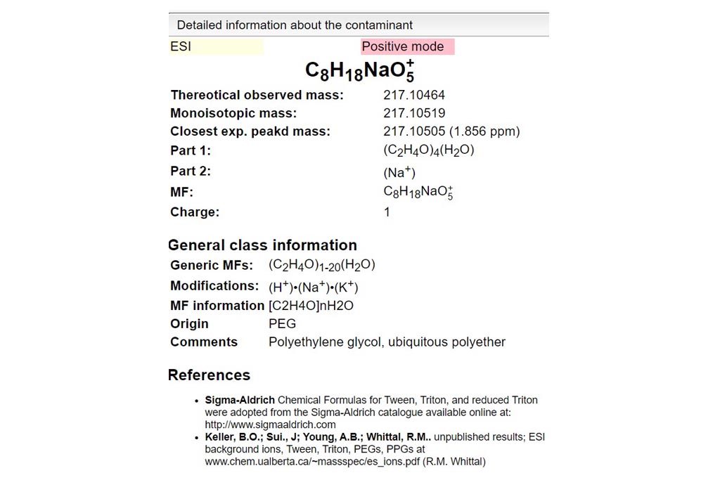
Info view

The Info box window shows details for the table-selected ion such as its name, monoisotopic mass,  molecular formula, charge and ionization adduct. You can find as well the theoretical monoisotopic mass and the closest m/z experimental data. Below this window, you’ll find the general information (which should be included during step 3) and the reference defined in the custom module.

Resuts 4

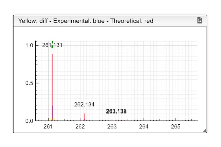
Similarity view

The Similarity box window displays the matching of theoretical isotopic pattern to experimental spectrum for the selected peaks with differences in the intensity of isotopologues highlighted in yellow. You can check our concept of similarity here.

[bsf-info-box icon_type=”custom” icon_img=”id^5079|url^https://ms.epfl.ch/wp-content/uploads/2020/05/equipo-contacta-con-nostros-transparente.png|caption^null|alt^null|title^equipo-contacta-con-nostros-transparente|description^null” img_width=”250″ title=”Do you want to share your results in this page?” heading_tag=”span” pos=”left” title_font_style=”font-weight:bold;” title_font_size=”desktop:22px;” title_font_color=”#333333″]The ISIC-EPFL MS team will be delighted to share your updates in ms.epfl.ch! If you want to describe your project using any of our free tools and share your results, you can publish a post describing the project & results and/or once published we could include in our mstoolbox references page. You can also share any of your learning materials contact us. In any case, If you want to be updated, follow us in twitter or linkedln.[/bsf-info-box]