[ultimate_heading main_heading=”Web-based application for polymer analysis mass spectrometry datasets” main_heading_margin=”margin-bottom:10px;” main_heading_style=”font-weight:bold;” main_heading_font_size=”desktop:50px;” main_heading_line_height=”desktop:60px;”]MSPolyCalc is a free and open access application for interpretation of complex polymers mass spectra. MSPolyCalc offers new functionalities such as determination of polymer distribution, molecular formula identification and similarity calculations for each peak assignment. The software was successfully tested with both high and low resolution mass spectrometers. You can read the paper here.[/ultimate_heading]
app-7
Generate the Molecular formula of your polymer with the ``small molecule`` applications.
Details
app-8
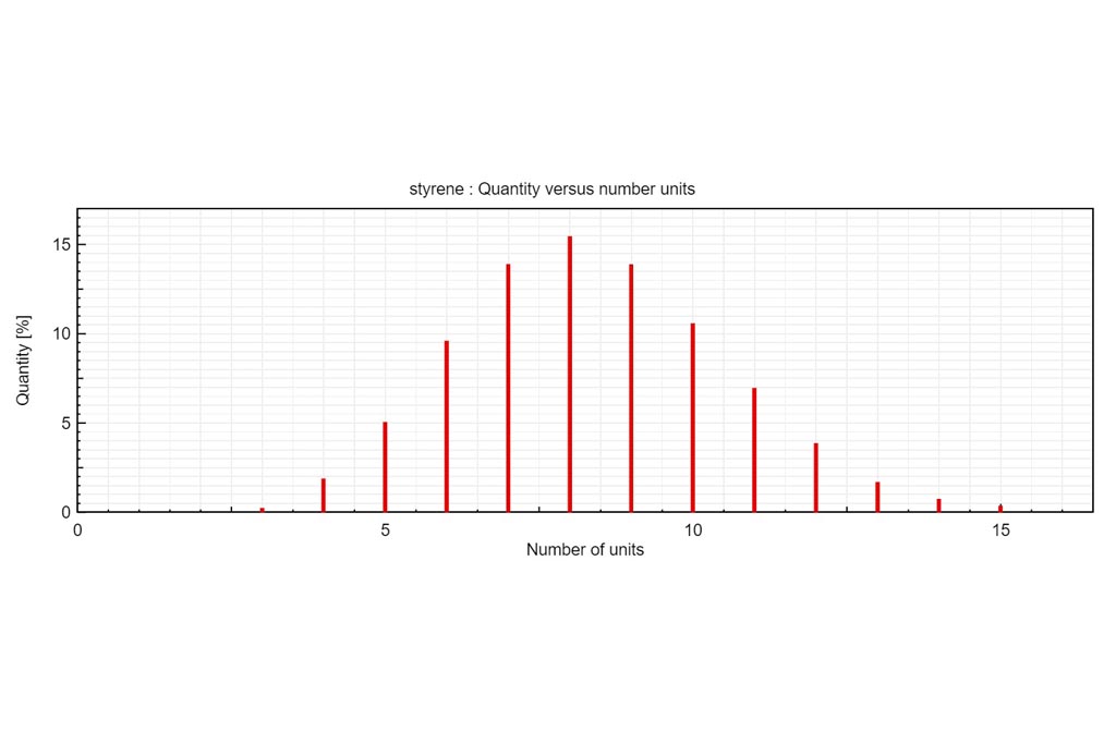
Advanced analysis of polymer mass spectra, with automatic peak picking and ion assignment.
Details
app-index-app2
Other open access applications for MS data interpretation.
Details
[ultimate_heading main_heading=”How to use MSPolyCalc step by step” main_heading_margin=”margin-bottom:10px;” main_heading_style=”font-weight:bold;” main_heading_font_size=”desktop:50px;” main_heading_line_height=”desktop:60px;”]The different Tab menus are described as follow : The Assign one is suitable for targeted analysis. The Explore Tab facilitates species identification for non-targeted analysis. Key background calculations can be tracked via the Monitor Tab. Via the Kendrick Tab, MSPolyCalc offers the possibility to generate Kendrick Mass Defect (KMD) plots and finally the Report Tab provides a summary of the MS analysis[/ultimate_heading]

STEP 1

Importing Experimental data

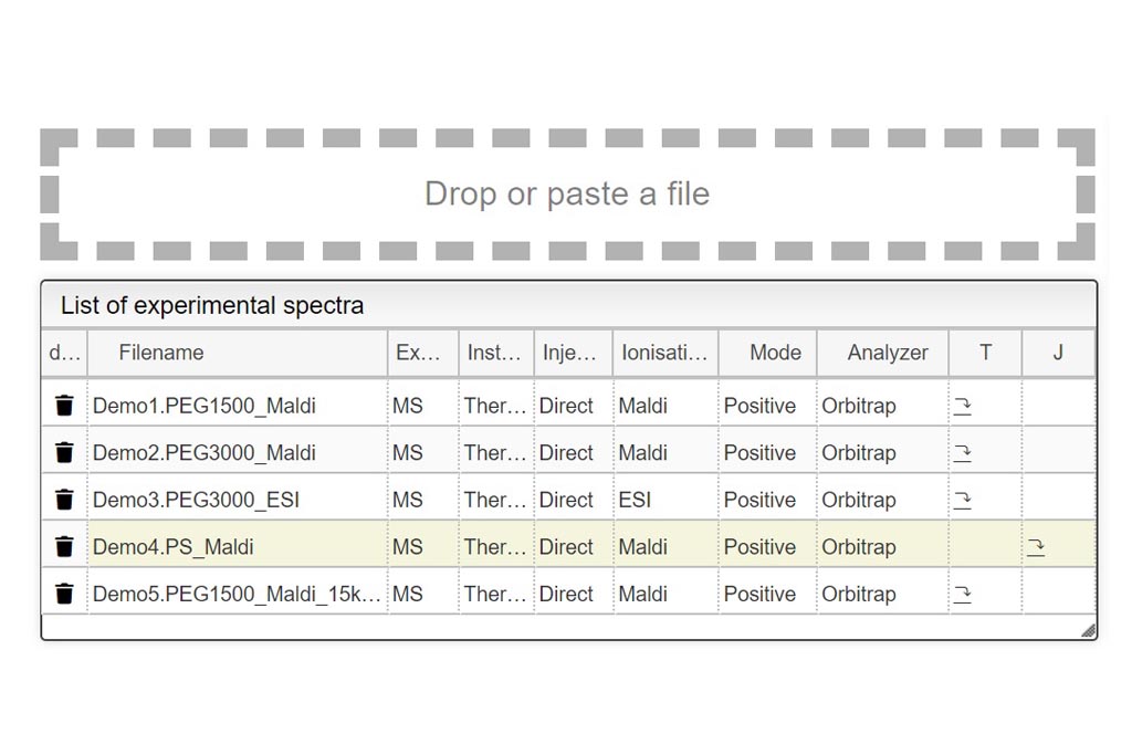
This tool can be either used in a LIMS or stand-alone. In the stand-alone mode you should either drag/drop your experimental spectrum as a tab-delimited text file or copy paste it (CTRL-V) while moving you mouse over the drop zone. The list of available spectra will be displayed in the table and you may click on one of them to display it.

STEP 2 (Automatic)

Automatic Peak Picking

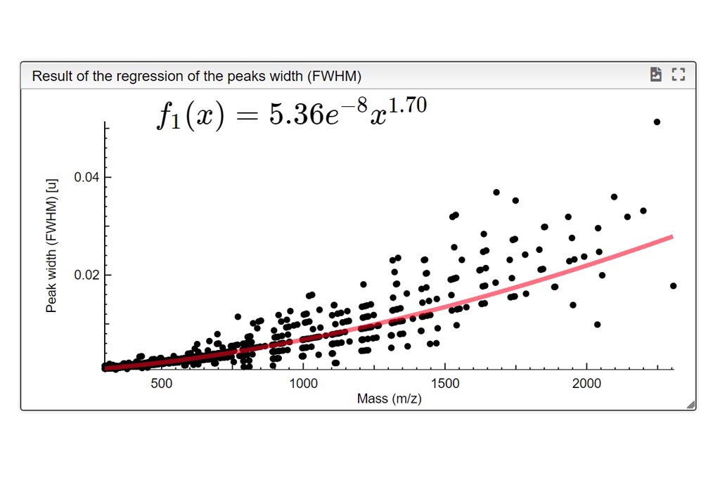
The application automatically performs a peak picking from loaded experimental spectra. It is important to notice that this function requires the experimental spectra to be plotted as profiles and not centroids. The spectral resolution typically decreases as m/z increases. Here, the application calculates a regression function f1(x) that fits the best the experimental data. This function is then automatically taken into account for the calculation of similarity scores as well as for the recalibration process, both available in the Assign tab. The regression function is displayed here for a polystyrene spectra, PS_MALDI, available as an example in the list of experimental spectra. 

STEP 3

Polymer selection and description

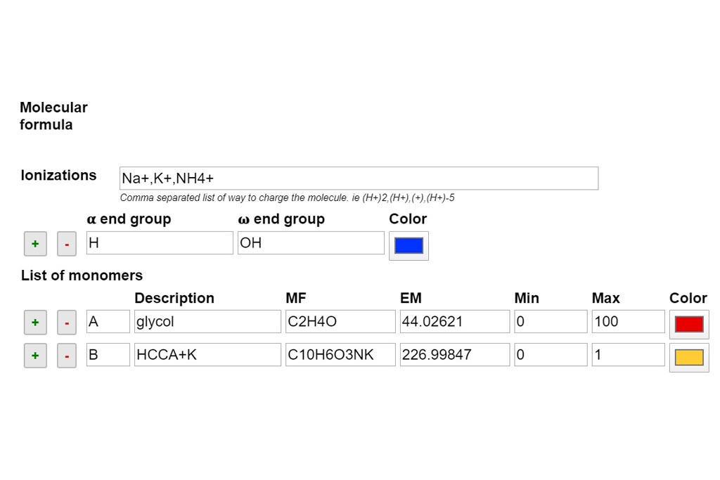
Then, you need to define the main physical properties of targeted polymers such as the end groups, the repeating units (list of monomers) and the adducts (ionization). This combination will generate a list of possible polymer ions. The displayed example for polymer selection is a PEG polymer, PEG1500_Maldi, available in the list of experimental spectra.

STEP 4

Molecular Formula filtering

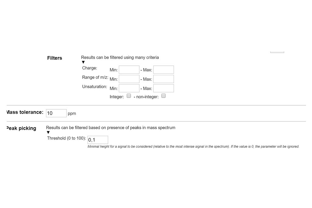
The user can fine-tune the obtained molecular formula in step 4 by different criteria such as the charge, the experimental m/z or the unsaturation (double bond equivalent).  This function provides high flexibility  and allows users to broadly screen a range of expected MF and hypotheses, eventually simulating termination reactions, oxidation, or complex mixtures, among others. The PEG3000 polymer is displayed as an example, available in the list of experimental data. 

STEP 5

Experimental filtering

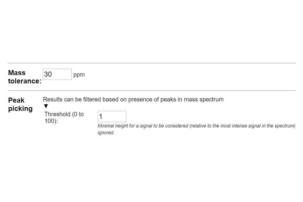
Two experimental filters should be defined. Firstly, we need to set the authorized experimental mass error in ppm (around 30 ppm in our MALDI experiments) and then set the experimental relative peak intensity threshold (0 to 100). Shown  example is  PEG3000, available in the list of experimental data. 

STEP 5

Select the matching threshold

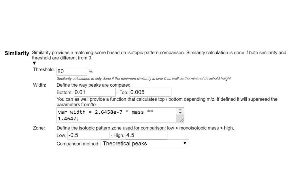
As mentioned above in section 2, peak selection is implemented automatically by the software after uploading of the experimental spectrum. Simultaneously and automatically, a regression is employed to describe the evolution of the full width at half maximum peak height (FWHM, i.e. resolution) as a function of m/z. The resulting regression function – identified as f1 – can be visualized in the Monitor Tab and will be used for the similarity calculations. You need as well to set a similarity threshold (typically 70-80%).Then the comparison zone should be adjusted based on the complexity of the expected isotopic pattern. Check our comparison method in the glossary. 

STEP 6 (Optional)

Recalibrate and reAssign

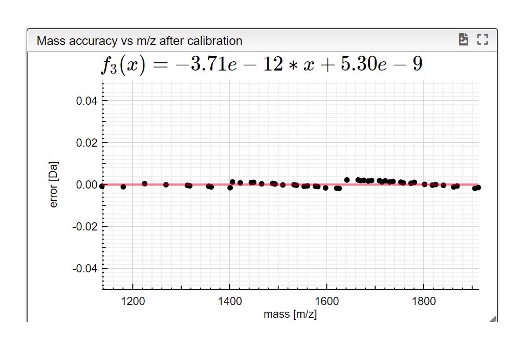
Once the calculation is done (a few seconds), if at least 10 isotopic distributions match the theoretical ones with more than 95% similarity) then mass accuracy is plotted based on m/z on the Monitor tab. A linear regression can be performed by clicking recalibrate m/z and results can be viewed on the Monitor tab. Then, again optionally, you can click recalibrate and reassign peaks in a few seconds. You can look at our PEG3000 example of recalibration, available in the list of experimental spectra. 

[ultimate_heading main_heading=”Different output views in MSPolyCalc” main_heading_margin=”margin-bottom:10px;” main_heading_style=”font-weight:bold;” main_heading_font_size=”desktop:35px;” main_heading_line_height=”desktop:60px;”][/ultimate_heading]

Resuts 1

List of fragments view

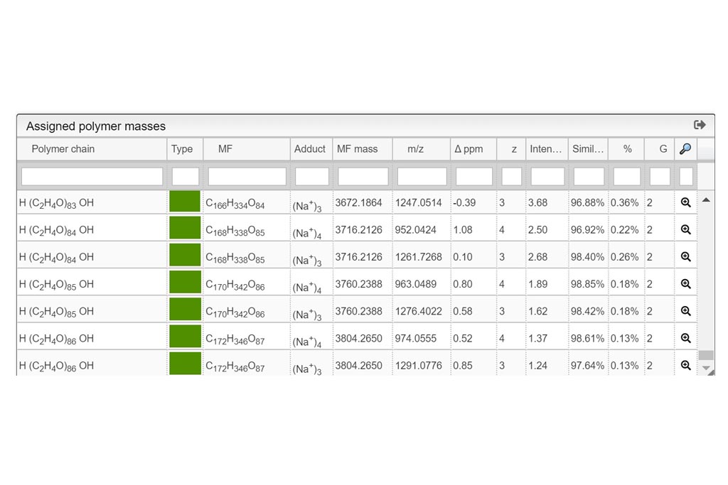
A detailed list of assigned polymer ions is given in Results 1. You can see the type of fragmentation, the molecular formula and its ionization form. You can see as well the Molecular formula monoisotopic peak (without ionization), the final monoisotopic mass including the charge and other interesting values such as the mass error (ppm), the similarity and the relative abundance. All peaks are integrated automatically and the relative abundance column provides a semi quantitative value of species importance. Peak integrals are also used to quantify the amount of assigned signal.

Resuts 2

Mass spectra view

Mass spectra view displays the experimental peaks (in red) overlaid with the matched theoretical ones (in blue). Identified ions are assigned and color-coded on the top with the charge in gray. You can select a single peak in the table view (Results 1) and it will be highlighted in this view (in yellow). It is possible to zoom (left button), de-zoom (double left button) and show the full screen (option bar at the top of the view). The content of this view can be either printed or exported as SVG file (option bar). The PEG3000 example view after recalibration is shown in the figure.

Resuts 3

Info view

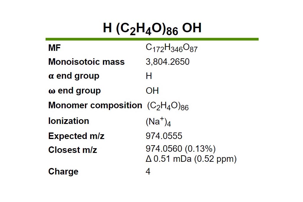
The Info view displays a summary of the ion features at the cursor position. This becomes particularly convenient when highlighting the position of polymer chains ionized under several adduct forms. This view shows the molecular formula, monoisotopic mass, end groups, charge, ionization adduct and monomer composition. You find as well the theoretical monoisotopic mass and the closest m/z experimental data. Below this window, the assigned quantity, the number of distinct ions found and their percentage of the total intensity are shown. The total amount of theoretically possible fragments based on selected combinations is displayed as well. One example of the PEG3000 identified ion is shown in the figure and the spectrum available in the list of experimental spectra.

Resuts 4

Similarity view

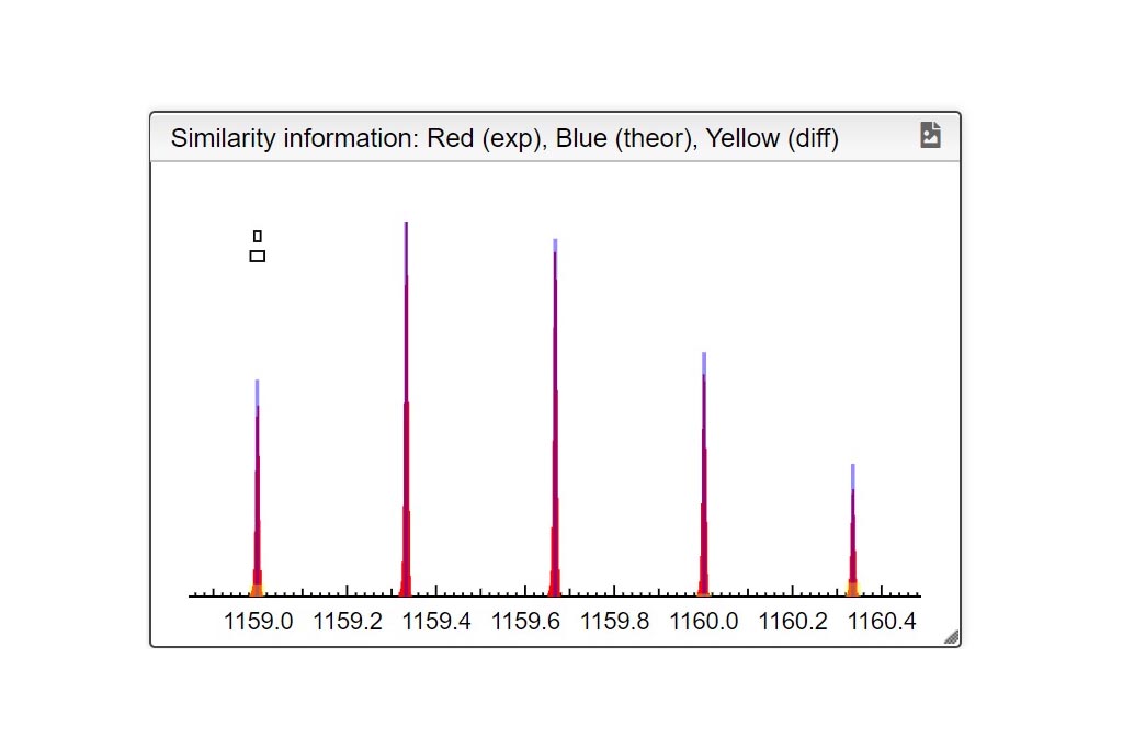
The Similarity box window displays the matching of theoretical isotopic pattern to experimental spectrum for the selected peak with differences in the intensity of isotopologues highlighted in yellow. You can check our concept of similarity here. Similarity calculation is shown for one identified ion of the PEG3000, example available in the list of experimental spectra. 

Resuts 5

Kendrick View

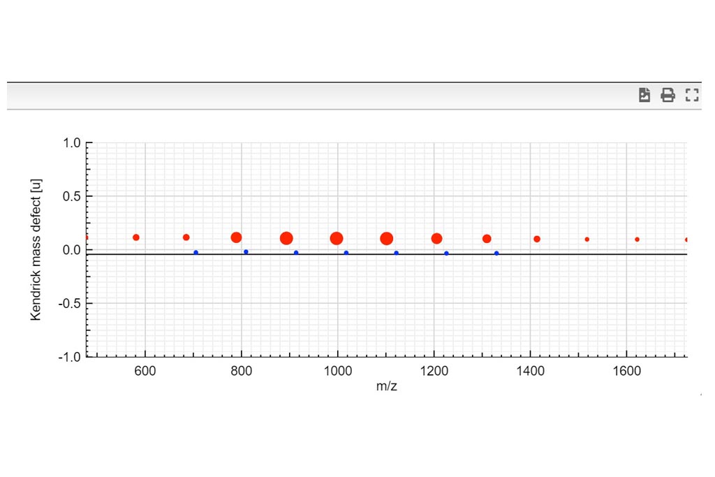
Kendrick mass defect plots were integrated in MSPolyCalc from the perspective of unravelling spectra complexity by offering a correlative approach. Two options are available. On one hand, the m/z KMD plot is determined from experimental m/z values (referring to [M+Na]+ for example). It yields a representative picture of the experimental mass spectrum, with different split distributions of same chemical composition but different ionization adduct. On another hand, a simplified KMD plot, named “deconvoluted” KMD plot can be plotted. In this case, mass defects are calculated from the MF masses, thus referring to the neutral species [M], and neglecting the contribution of the ionization adducts. Kendrick Tab is interactive and moving the mouse cursor over the plots controls what the Info Box displays.

Resuts 6

Report View

MSPolyCalc provides a summary of the polymer MS analysis and you can build a clear and printable output document.

[bsf-info-box icon_type=”custom” icon_img=”id^5079|url^https://ms.epfl.ch/wp-content/uploads/2020/05/equipo-contacta-con-nostros-transparente.png|caption^null|alt^null|title^equipo-contacta-con-nostros-transparente|description^null” img_width=”250″ title=”Do you want to share your results in this page?” heading_tag=”span” pos=”left” title_font_style=”font-weight:bold;” title_font_size=”desktop:22px;” title_font_color=”#333333″]The ISIC-EPFL MS team will be delighted to share your updates in ms.epfl.ch! If you want to describe your project using any of our free tools and share your results, you can publish a post describing the project & results and/or once published we could include in our mstoolbox references page. You can also share any of your learning materials contact us. In any case, If you want to be updated, follow us in twitter or linkedln.[/bsf-info-box]